Service area analysis — determining which geographic areas fall within reach of a facility, transit stop, or resource — is one of the most common tasks in applied spatial analysis. Retail site selection, transit accessibility modelling, emergency response planning, and delivery zone optimisation all depend on answering the same fundamental question: from this location, what territory can be reached?
Traditional approaches use circular buffers (drawing a radius around a point) or network-based isochrones (computing travel-time polygons). Both have limitations. Circular buffers ignore the shape of the road network and produce the same result everywhere on Earth, which sounds consistent but actually isn’t: a buffer drawn at high latitudes covers far more real-world area than one drawn near the equator. Network isochrones are accurate but computationally expensive and require access to routing infrastructure.
H3’s k-ring analysis offers a middle path: hexagonal catchment areas that are consistent in shape, scale efficiently across resolution levels, and require no routing infrastructure. They’re particularly useful for rapid prototyping, large-scale regional analysis, and anywhere you need spatial buffers that behave predictably.
How K-Ring Analysis Works
H3 represents the Earth as a discrete grid of hexagons. Each hexagon has exactly six neighbours at an equal distance — unlike squares, where corner neighbours are further away than edge neighbours. This consistency makes hexagonal grids ideal for neighbourhood analysis.
gridDisk(center, k) returns all hexagons within k steps of the center — the hexagonal equivalent of a filled circle.
gridRing(center, k) returns only the hexagons at exactly k steps away — the hexagonal equivalent of a ring or annulus.
const center = h3.latLngToCell(51.505, -0.09, 8); // resolution 8

const disk    = h3.gridDisk(center, 3);   // all cells within 3 steps: 1 + 6 + 12 + 18 = 37 cells
const ring3   = h3.gridRing(center, 3);  // only the cells at exactly 3 steps: 18 cells

// The count of cells in a disk of radius k is: 3k² + 3k + 1
// The count of cells in ring k is: 6k (for k > 0)
console.log(`Disk: ${disk.length} cells`);  // 37
console.log(`Ring 3: ${ring3.length} cells`); // 18
The formula 3k² + 3k + 1 gives the total number of cells in a disk of radius k — useful for estimating coverage before running the query.
Setting Up the Demo Environment
The demos in this tutorial use Leaflet for map rendering and H3.js for all spatial operations:
<!DOCTYPE html>
<html>
<head>
    <title>H3 Catchment Analysis</title>
    <link rel="stylesheet" href="https://unpkg.com/leaflet@1.9.4/dist/leaflet.css" />
    <style>
        #map { height: 480px; width: 100%; border-radius: 8px; }
        .controls { margin: 12px 0; display: flex; gap: 20px; align-items: center; flex-wrap: wrap; }
        .info-panel {
            background: #f0f4f8;
            padding: 10px 14px;
            border-radius: 6px;
            font-family: monospace;
            font-size: 13px;
            margin-top: 10px;
            min-height: 40px;
        }
    </style>
</head>
<body>
    <div class="controls">
        <label>K (ring radius):
            <input type="range" id="kValue" min="1" max="12" value="3" />
            <span id="kDisplay">3</span>
        </label>
        <label>Resolution:
            <input type="range" id="resolution" min="6" max="10" value="8" />
            <span id="resDisplay">8</span>
        </label>
    </div>
    <div id="map"></div>
    <div class="info-panel" id="info">Click anywhere on the map to place a catchment centre.</div>

    <script src="https://unpkg.com/leaflet@1.9.4/dist/leaflet.js"></script>
    <script src="https://unpkg.com/h3-js@4.3.0/dist/h3-js.umd.js"></script>
</body>
</html>
Interactive Demo 1: Expanding Catchment Rings
This demo lets you place a catchment centre anywhere on the map and visualise the expanding hexagonal rings around it. Each ring is coloured differently so you can see exactly which areas fall at which distance from the centre.
What you’ll learn:
K-ring analysis reveals the spatial neighbourhood structure around any point. You’ll observe that hexagonal rings expand consistently in all directions, unlike circular buffers that can intersect grid boundaries awkwardly. The colouring by ring distance gives you an immediate visual sense of spatial accessibility — the kind of graduated catchment map used in retail site analysis and transit planning.
How to use:
Click anywhere on the map to set a catchment centre. Use the K slider to expand or shrink the catchment radius. Use the resolution slider to change hexagon size — notice how the coverage area in km² changes as both K and resolution change. The info panel shows the total cells, estimated coverage area, and the approximate real-world radius.
Key concepts demonstrated:
gridDisk computes the full catchment (all cells within k steps). gridRing isolates individual distance rings, which is useful for modelling travel cost zones. Consistent Neighbourhood Structure means the ring at k=3 always contains exactly 18 cells, regardless of where on Earth the centre is located — a property that squares do not have.
const map = L.map('map').setView([51.505, -0.09], 12);
L.tileLayer('https://{s}.tile.openstreetmap.org/{z}/{x}/{y}.png', {
attribution: '© OpenStreetMap contributors'
}).addTo(map);
// Colour palette for concentric rings (centre → outer)
const ringColors = [
'#c0392b', // k=0 (centre)
'#e67e22', // k=1
'#f1c40f', // k=2
'#2ecc71', // k=3
'#1abc9c', // k=4
'#3498db', // k=5
'#9b59b6', // k=6
'#34495e', // k=7+
];
let catchmentLayers = [];
let centerMarker = null;
function getColor(k) {
return ringColors[Math.min(k, ringColors.length - 1)];
}
function renderCatchment(centerH3, k, resolution) {
// Clear previous layers
catchmentLayers.forEach(l => map.removeLayer(l));
catchmentLayers = [];
let totalCells = 0;
// Draw rings from outside in so the centre is visible on top
for (let ring = k; ring >= 0; ring--) {
const cells = ring === 0
? [centerH3]
: h3.gridRing(centerH3, ring);
cells.forEach(h3Index => {
const boundary = h3.cellToBoundary(h3Index, true);
const layer = L.polygon(boundary, {
color: '#ffffff',
weight: 0.5,
fillColor: getColor(ring),
fillOpacity: ring === 0 ? 0.9 : 0.45
}).addTo(map);
layer.bindTooltip(`Ring ${ring} — ${ring} step${ring !== 1 ? 's' : ''} from centre`, { sticky: true });
catchmentLayers.push(layer);
});
totalCells += cells.length;
}
// Stats
const cellArea = h3.getHexagonAreaAvg(resolution, h3.UNITS.km2);
const totalArea = totalCells * cellArea;
// Approximate radius: area of disk = π r² → r = sqrt(area/π)
const approxRadius = Math.sqrt(totalArea / Math.PI).toFixed(2);
document.getElementById('info').innerHTML =
`<strong>K:</strong> ${k} | ` +
`<strong>Cells:</strong> ${totalCells} (= 3×${k}²+3×${k}+1) | ` +
`<strong>Coverage:</strong> ~${totalArea.toFixed(2)} km² | ` +
`<strong>Approx radius:</strong> ~${approxRadius} km`;
}
const kSlider = document.getElementById('kValue');
const resSlider = document.getElementById('resolution');
function refresh() {
if (!window.currentCenter) return;
const resolution = parseInt(resSlider.value);
const k = parseInt(kSlider.value);
const centerH3 = h3.latLngToCell(window.currentCenter.lat, window.currentCenter.lng, resolution);
renderCatchment(centerH3, k, resolution);
}
kSlider.addEventListener('input', () => {
document.getElementById('kDisplay').textContent = kSlider.value;
refresh();
});
resSlider.addEventListener('input', () => {
document.getElementById('resDisplay').textContent = resSlider.value;
refresh();
});
map.on('click', e => {
window.currentCenter = e.latlng;
if (centerMarker) map.removeLayer(centerMarker);
centerMarker = L.circleMarker(e.latlng, { radius: 5, color: '#c0392b', fillColor: '#c0392b', fillOpacity: 1 }).addTo(map);
refresh();
});One subtle but important property is visible here: every hexagonal ring at distance k contains exactly 6k cells. This means the catchment grows predictably — you can compute exactly how many cells (and thus how much area) will be included before performing any spatial operation.
Grid Distance Between Two Points
Beyond building catchments around a single centre, H3 can compute the grid distance between any two hexagons — how many steps it takes to travel from one to another through the hexagonal grid.
// How far is one location from another, in grid steps?
function hexDistance(lat1, lng1, lat2, lng2, resolution) {
    const cell1 = h3.latLngToCell(lat1, lng1, resolution);
    const cell2 = h3.latLngToCell(lat2, lng2, resolution);
    return h3.gridDistance(cell1, cell2);
}

// Example: distance from St Paul's to Tate Modern at resolution 9
const steps = hexDistance(51.5138, -0.0984, 51.5076, -0.0994, 9);
console.log(`Grid distance: ${steps} steps`);
Grid distance is fast (O(1)) and consistent. Unlike Euclidean distance, it accounts for the discrete structure of the grid, making it more appropriate for problems where movement happens in steps rather than continuously.
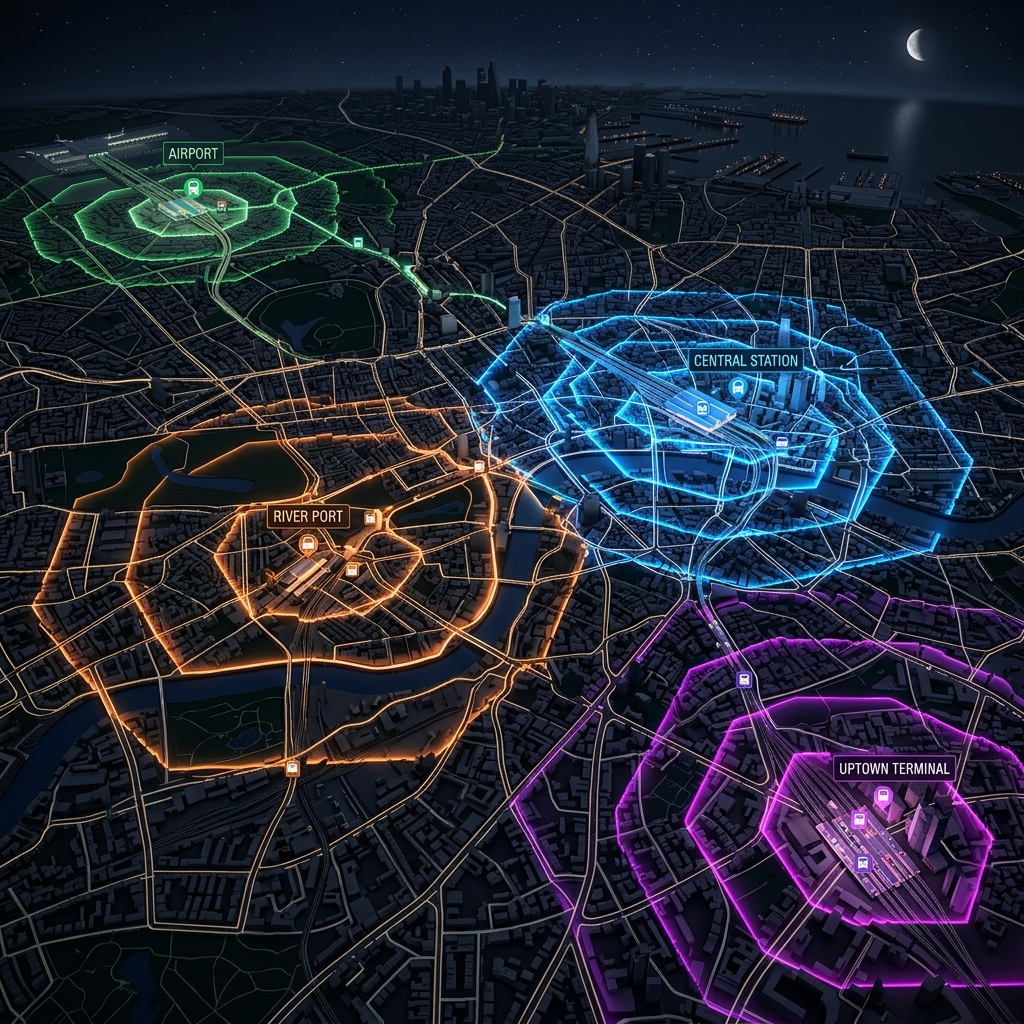
Interactive Demo 2: Multi-Source Catchment Overlap
Real-world service area analysis often involves multiple sources — several retail locations, multiple transit stops, or a set of emergency facilities. Understanding where catchments overlap reveals gaps, redundancy, and competitive boundaries.
What you’ll learn:
When two catchments overlap, cells belong to multiple service areas simultaneously. Counting how many sources cover each cell reveals coverage redundancy (cells served by multiple sources) and gaps (cells outside all catchments). This is a core technique in facility location optimisation.
Key concepts demonstrated:
Set Operations on H3 Cells work naturally with standard JavaScript Set and Map data structures — H3 indices are just strings, so intersection, union, and difference are straightforward. Coverage Density counts how many sources cover each hexagon, which you can render as a choropleth. Competitive Boundary Detection finds cells where two or more catchments meet.
// Place two service centres and compute their catchments
const centres = [
    { lat: 51.515, lng: -0.090 }, // Centre A
    { lat: 51.495, lng: -0.120 }  // Centre B
];

const resolution = 8;
const k = 5;

const catchmentMaps = centres.map(({ lat, lng }) => {
    const centerCell = h3.latLngToCell(lat, lng, resolution);
    return new Set(h3.gridDisk(centerCell, k));
});

// Count how many catchments cover each cell
const coverageCount = new Map();
catchmentMaps.forEach(catchment => {
    catchment.forEach(cell => {
        coverageCount.set(cell, (coverageCount.get(cell) || 0) + 1);
    });
});

// Identify overlap zone (covered by both)
const overlapCells = [...coverageCount.entries()]
    .filter(([, count]) => count >= 2)
    .map(([cell]) => cell);

console.log(`Total unique cells covered: ${coverageCount.size}`);
console.log(`Overlap cells: ${overlapCells.length}`);

// Render with coverage-count colouring
const overlapColors = { 1: '#3498db', 2: '#e74c3c' };

coverageCount.forEach((count, h3Index) => {
    const boundary = h3.cellToBoundary(h3Index, true);
    L.polygon(boundary, {
        fillColor: overlapColors[count] || '#9b59b6',
        fillOpacity: count === 2 ? 0.7 : 0.35,
        color: 'none',
        weight: 0
    }).addTo(map);
});
The overlap computation is pure set arithmetic operating on H3 index strings — no geometric intersection required. This is one of H3’s most powerful properties: spatial operations that traditionally require expensive polygon intersection libraries reduce to simple string-based set operations.
Choosing the Right Resolution for Catchment Analysis
The relationship between k and real-world distance depends on the resolution:
| Resolution | Avg cell width | k=1 (6 cells) | k=5 (91 cells) | k=10 (331 cells) |
|---|---|---|---|---|
| 6 | ~36 km | ~36 km | ~180 km | ~360 km |
| 7 | ~13 km | ~13 km | ~65 km | ~130 km |
| 8 | ~5 km | ~5 km | ~25 km | ~50 km |
| 9 | ~2 km | ~2 km | ~10 km | ~20 km |
| 10 | ~0.7 km | ~0.7 km | ~3.5 km | ~7 km |
For walkability analysis, resolution 10 with k=5–15 gives you pedestrian-scale catchments. For regional transit analysis, resolution 7 or 8 is more appropriate. For national-level facility planning, resolution 5 or 6.
A general heuristic: choose the resolution where one hexagon is roughly the size of your minimum meaningful unit, then set k to match your desired catchment radius.
Practical Applications
H3 catchment analysis is applied across a range of domains:
Retail site selection: Compare the population covered by alternative store locations at k=10 (roughly 5 km at resolution 8). Sites with overlapping catchments compete for the same customers.
Transit accessibility: For each transit stop, compute a walkability catchment at resolution 10, k=8 (roughly 5 minute walk). Cells outside all catchments have poor transit access.
Emergency response: Model which areas fall within a 5-minute drive of each station using k-ring proxies, then identify under-served cells for new facility placement.
Delivery zone optimisation: Assign each cell to its nearest depot using gridDistance, creating Voronoi-like zones that partition the entire coverage area without gaps.
Next Steps
K-ring analysis gives you hexagonal buffers; H3’s hierarchy gives you multi-resolution analysis. The next post in this series covers H3’s parent-child relationships and compaction algorithm — how to represent the same spatial area at different scales without redundancy, and why this matters for spatial database design and efficient data transmission.