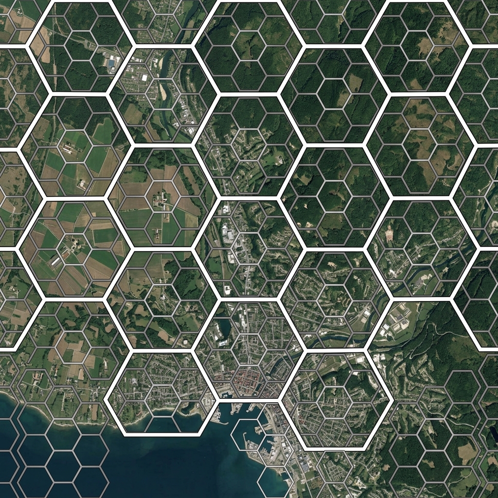
Every H3 hexagon contains exactly seven children at the next finer resolution level. Not approximately seven — exactly seven, for every cell, at every resolution, everywhere on Earth (with a small number of pentagon exceptions at the boundaries of the twelve base faces, but these can be handled uniformly with h3.isPentagon()).
This seven-to-one ratio is the defining property of H3’s hierarchical design. It means you can move between resolutions analytically without any loss of information, represent the same spatial area at multiple scales using a consistent index structure, and compress sets of fine-resolution cells into their coarser parents when all seven children are present. This last operation — compaction — is where H3’s hierarchy becomes practically powerful.
Understanding the Hierarchy
H3 supports sixteen resolution levels (0–15). Resolution 0 cells cover approximately 4,250 km² each; resolution 15 cells cover less than a square metre. Each step down in resolution divides cells by seven:
Resolution 0: ~4,250 km² per cell
Resolution 1: ~607 km² per cell  (÷ 7)
Resolution 2: ~86.7 km² per cell (÷ 7)
Resolution 3: ~12.4 km² per cell (÷ 7)
...
Resolution 9: ~0.105 km² per cell
Resolution 15: ~0.895 m² per cell
H3 provides direct functions for navigating this hierarchy:
// Move up: get the resolution-6 parent of a resolution-9 cell
const cell9 = h3.latLngToCell(51.505, -0.09, 9);
const parent6 = h3.cellToParent(cell9, 6);
console.log(parent6); // An H3 index at resolution 6

// Move down: get all resolution-10 children of a resolution-8 cell
const cell8 = h3.latLngToCell(51.505, -0.09, 8);
const children10 = h3.cellToChildren(cell8, 10); // 7² = 49 cells
console.log(children10.length); // 49

// Skip multiple levels: resolution-8 cell has 7² = 49 resolution-10 children
// and 7³ = 343 resolution-11 children
const children11 = h3.cellToChildren(cell8, 11);
console.log(children11.length); // 343
When you skip multiple resolution levels, the number of children grows as 7^(targetRes - sourceRes). A single resolution-6 cell has 7^3 = 343 resolution-9 children and 7^6 = 117,649 resolution-12 children.
The Compaction Algorithm
Compaction answers a simple question: given a set of H3 cells, what is the minimum set of cells (possibly at mixed resolutions) that covers exactly the same area?
If all seven children of a parent cell are present in your set, you can replace them with just the parent — saving six entries. H3’s compactCells function applies this recursively from the finest resolution upward:
// Generate a set of fine-resolution cells covering a region
const centerCell = h3.latLngToCell(51.505, -0.09, 9);
const disk = h3.gridDisk(centerCell, 10); // 331 cells at resolution 9

// Compact: replace complete sets of 7 siblings with their parent
const compacted = h3.compactCells(disk);
console.log(`Original: ${disk.length} cells`);
console.log(`Compacted: ${compacted.length} cells`);
// Compacted will be significantly smaller, at mixed resolutions

// Uncompact back to a uniform resolution
const uncompacted = h3.uncompactCells(compacted, 9);
console.log(`Uncompacted: ${uncompacted.length} cells`); // Same as disk
For a circular disk, compaction rates vary: cells near the centre form complete parent groups and compact aggressively, whilst cells near the boundary are incomplete and remain at the original resolution. The result is a mixed-resolution set that is mathematically equivalent to the original but uses far fewer entries.
Setting Up the Interactive Demo
The following demos use Leaflet and H3.js, both loaded from CDN:
<!DOCTYPE html>
<html>
<head>
<title>H3 Hierarchy Explorer</title>
<link rel="stylesheet" href="https://unpkg.com/leaflet@1.9.4/dist/leaflet.css" />
<style>
#map { height: 480px; width: 100%; border-radius: 8px; }
.controls { margin: 12px 0; display: flex; gap: 16px; align-items: center; flex-wrap: wrap; }
.info-panel {
background: #f0f4f8;
padding: 10px 14px;
border-radius: 6px;
font-family: monospace;
font-size: 13px;
margin-top: 10px;
}
.legend { margin-top: 8px; font-size: 12px; font-family: monospace; }
.swatch {
display: inline-block;
width: 14px; height: 14px;
border-radius: 3px;
margin-right: 4px;
vertical-align: middle;
}
</style>
</head>
<body>
<div class="controls">
<label>Base Resolution:
<input type="range" id="baseRes" min="5" max="9" value="8" />
<span id="baseResDisplay">8</span>
</label>
<label>Disk radius (k):
<input type="range" id="kValue" min="1" max="8" value="4" />
<span id="kDisplay">4</span>
</label>
<label>
<input type="checkbox" id="showCompact" checked />
Show compact cells
</label>
</div>
<div id="map"></div>
<div class="info-panel" id="info">Click on the map to place a centre hexagon.</div>
<div class="legend">
<span class="swatch" style="background:#3498db"></span>Fine resolution (original)
<span class="swatch" style="background:#e74c3c"></span>Coarser parent (compacted)
<span class="swatch" style="background:#f39c12"></span>Boundary (uncompactable)
</div>
<script src="https://unpkg.com/leaflet@1.9.4/dist/leaflet.js"></script>
<script src="https://unpkg.com/h3-js@4.3.0/dist/h3-js.umd.js"></script>
</body>
</html>Interactive Demo 1: Parent-Child Hierarchy Explorer
Click on the map to select a hexagon, then use the resolution slider to navigate up and down the hierarchy. Watch how the selected cell’s parent covers the same area as seven children, and how the parent’s parent covers the area of 49 cells at the original resolution.
What you’ll learn:
Navigating the H3 hierarchy shows concretely how spatial precision and coverage area trade off. Moving to a coarser parent reduces the number of cells needed to represent an area, at the cost of spatial precision. This trade-off is fundamental to efficient spatial data storage and multi-resolution analytics.
How to use:
Click on the map to select a base cell (shown in blue). The cell’s parent chain is displayed in progressively lighter shades up to the configured base resolution. The info panel shows the selected cell’s index, its resolution, and its parent at each level.
Key concepts demonstrated:
cellToParent moves up the hierarchy by increasing coarseness. cellToChildren moves down by subdividing each cell into seven. Resolution Jump demonstrates that skipping multiple levels is equivalent to applying cellToParent repeatedly — the result is identical.
const map = L.map('map').setView([51.505, -0.09], 12);
L.tileLayer('https://{s}.tile.openstreetmap.org/{z}/{x}/{y}.png', {
attribution: '© OpenStreetMap contributors'
}).addTo(map);
let hierarchyLayers = [];
// Colours for each level above the selected cell
const levelColors = ['#2980b9', '#1abc9c', '#e67e22', '#e74c3c', '#9b59b6'];
function renderHierarchy(lat, lng, fineRes) {
hierarchyLayers.forEach(l => map.removeLayer(l));
hierarchyLayers = [];
const fineCell = h3.latLngToCell(lat, lng, fineRes);
const minRes = Math.max(0, fineRes - 4);
// Render from coarsest to finest so finer cells sit on top
for (let res = minRes; res <= fineRes; res++) {
const levelDepth = fineRes - res; // 0 = fine, 4 = coarsest
const cell = h3.cellToParent(fineCell, res);
const boundary = h3.cellToBoundary(cell, true);
const color = levelColors[Math.min(levelDepth, levelColors.length - 1)];
const layer = L.polygon(boundary, {
color: color,
weight: levelDepth === 0 ? 3 : 1,
fillColor: color,
fillOpacity: levelDepth === 0 ? 0.6 : 0.15,
dashArray: levelDepth > 0 ? '4,4' : null
}).addTo(map);
const area = h3.getHexagonAreaAvg(res, h3.UNITS.km2).toFixed(3);
layer.bindTooltip(`Resolution ${res} — ${area} km²`, { sticky: true });
hierarchyLayers.push(layer);
}
// Display parent chain in info panel
let infoHtml = `<strong>Selected cell (res ${fineRes}):</strong> ${fineCell}<br/>`;
for (let res = fineRes - 1; res >= minRes; res--) {
const parent = h3.cellToParent(fineCell, res);
const childCount = Math.pow(7, fineRes - res);
infoHtml += `<strong>Parent res ${res}:</strong> ${parent} (contains ${childCount} res-${fineRes} children)<br/>`;
}
document.getElementById('info').innerHTML = infoHtml;
}
map.on('click', e => {
const baseRes = parseInt(document.getElementById('baseRes').value);
renderHierarchy(e.latlng.lat, e.latlng.lng, baseRes);
});
document.getElementById('baseRes').addEventListener('input', function() {
document.getElementById('baseResDisplay').textContent = this.value;
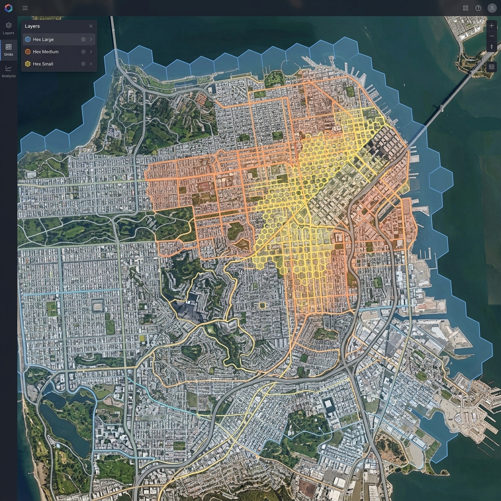
});Interactive Demo 2: Compaction Visualiser
This demo generates a disk of hexagons at a fine resolution and shows which cells compact to coarser parents (displayed in red) and which remain at the original resolution because their sibling set is incomplete (displayed in blue or orange).
What you’ll learn:
Compaction is not uniform across a spatial region. Cells near the centre of a convex shape compact most aggressively because all seven siblings are typically present. Cells near the boundary often have missing siblings outside the region boundary, so they cannot compact. This is why compaction rates are highest for compact convex regions and lowest for irregular or boundary-heavy shapes.
Key concepts demonstrated:
compactCells reduces a uniform-resolution set to a mixed-resolution minimum cover. The resulting set is spatially equivalent but uses fewer entries. Resolution Mixing in the compacted output shows cells at different resolutions — coarser cells cover areas where all siblings were present, finer cells cover partial groups at boundaries. Compression Rate varies by shape: circular disks compact to 30–50% of the original size; irregular shapes may compact less.
const map = L.map('map').setView([51.505, -0.09], 12);
L.tileLayer('https://{s}.tile.openstreetmap.org/{z}/{x}/{y}.png', {
attribution: '© OpenStreetMap contributors'
}).addTo(map);
let compactLayers = [];
function renderCompaction(lat, lng, resolution, k, showCompact) {
compactLayers.forEach(l => map.removeLayer(l));
compactLayers = [];
const centerCell = h3.latLngToCell(lat, lng, resolution);
const diskCells = h3.gridDisk(centerCell, k);
const compacted = h3.compactCells(diskCells);
const diskSet = new Set(diskCells);
if (showCompact) {
// Show compacted representation with mixed-resolution colouring
compacted.forEach(h3Index => {
const boundary = h3.cellToBoundary(h3Index, true);
const cellRes = h3.getResolution(h3Index);
const isCoarser = cellRes < resolution;
const isBoundary = cellRes === resolution;
const color = isCoarser ? '#e74c3c' :
isBoundary ? '#f39c12' : '#3498db';
const layer = L.polygon(boundary, {
color: '#ffffff',
weight: 0.5,
fillColor: color,
fillOpacity: 0.65
}).addTo(map);
const area = h3.getHexagonAreaAvg(cellRes, h3.UNITS.km2).toFixed(4);
layer.bindTooltip(`Res ${cellRes} — ${area} km² ${isCoarser ? '(compacted parent)' : '(boundary cell)'}`, { sticky: true });
compactLayers.push(layer);
});
} else {
// Show original fine-resolution disk
diskCells.forEach(h3Index => {
const boundary = h3.cellToBoundary(h3Index, true);
const isCenter = h3Index === centerCell;
const layer = L.polygon(boundary, {
color: '#ffffff',
weight: 0.5,
fillColor: '#3498db',
fillOpacity: isCenter ? 0.9 : 0.5
}).addTo(map);
compactLayers.push(layer);
});
}
// Compression statistics
const compressedPercent = ((1 - compacted.length / diskCells.length) * 100).toFixed(1);
const coarserCount = compacted.filter(c => h3.getResolution(c) < resolution).length;
const boundaryCount = compacted.filter(c => h3.getResolution(c) === resolution).length;
document.getElementById('info').innerHTML =
`<strong>Original cells:</strong> ${diskCells.length} | ` +
`<strong>Compacted:</strong> ${compacted.length} cells (${compressedPercent}% reduction) | ` +
`<strong>Compacted parents:</strong> ${coarserCount} | ` +
`<strong>Boundary cells:</strong> ${boundaryCount}`;
}
let currentCenter = null;
function refresh() {
if (!currentCenter) return;
const res = parseInt(document.getElementById('baseRes').value);
const k = parseInt(document.getElementById('kValue').value);
const showCompact = document.getElementById('showCompact').checked;
renderCompaction(currentCenter.lat, currentCenter.lng, res, k, showCompact);
}
document.getElementById('baseRes').addEventListener('input', function() {
document.getElementById('baseResDisplay').textContent = this.value;
refresh();
});
document.getElementById('kValue').addEventListener('input', function() {
document.getElementById('kDisplay').textContent = this.value;
refresh();
});
document.getElementById('showCompact').addEventListener('change', refresh);
map.on('click', e => {
currentCenter = e.latlng;
refresh();
});Toggle the “Show compact cells” checkbox to compare the original fine-resolution representation against the compacted mixed-resolution version. Notice how the centre of the disk compacts most aggressively, whilst the ring of cells at the boundary cannot compact because their siblings outside the disk boundary are absent.
Why Compaction Matters in Practice
Compaction is particularly valuable in three scenarios:
Spatial database storage. Storing millions of fine-resolution H3 indices is expensive. Compacting before storage can reduce row counts by 40–60% for typical urban regions. Both BigQuery and PostgreSQL with the H3 extension support querying compacted cell sets directly.
API response payloads. When sending spatial coverage zones from server to client, compaction reduces payload size significantly. A delivery zone covering 50,000 resolution-10 cells might compact to 8,000 mixed-resolution cells — a 6× reduction in payload before any compression is applied.
Region membership testing. Checking whether a point falls within a region stored as compacted cells requires checking cellToParent(point_cell, res) at each resolution level present in the compacted set — still fast, and much more memory-efficient than storing every fine-resolution cell explicitly.
# Python: check if a point falls within a compacted region
import h3

def in_compacted_region(lat, lng, compacted_cells):
    # Group compacted cells by resolution
    by_res = {}
    for cell in compacted_cells:
        res = h3.get_resolution(cell)
        by_res.setdefault(res, set()).add(cell)

    # For each resolution present, check if the point's parent is in the set
    for res, cells in by_res.items():
        if h3.latlng_to_cell(lat, lng, res) in cells:
            return True
    return False
Pentagon Awareness
H3’s hierarchical structure has one important caveat: twelve cells at every resolution are pentagons, not hexagons. These arise from the mathematical requirement to tile a sphere — icosahedral symmetry forces twelve pentagonal faces at each resolution level.
Pentagons have five neighbours instead of six, and their parent-child relationships are slightly different (a pentagon has six children, not seven). For most practical analyses at resolution 8 and above, pentagons are rare enough to ignore, but robust code should handle them:
// Filter out pentagons if your analysis assumes hexagonal structure
const hexagons = cells.filter(cell => !h3.isPentagon(cell));

// Or count them for diagnostics
const pentagonCount = cells.filter(cell => h3.isPentagon(cell)).length;
console.log(`Pentagon cells in set: ${pentagonCount} of ${cells.length}`);
At resolution 9, there are 12 pentagons out of approximately 4.2 million cells — a frequency of roughly 0.0003%.
Combining Hierarchy with Density Analysis
The hierarchy becomes especially powerful when combined with density mapping (covered in the previous post in this series). Rather than choosing a fixed resolution upfront, you can analyse data at multiple resolutions simultaneously and present the coarsest level that still shows meaningful variation:
// Adaptive resolution: use fine resolution where data is dense,
// coarser resolution where data is sparse
function adaptiveResolution(points, targetCellsPerHex = 5) {
    let resolution = 5; // Start coarse

    while (resolution < 11) {
        const cellCounts = new Map();
        points.forEach(({ lat, lng }) => {
            const idx = h3.latLngToCell(lat, lng, resolution);
            cellCounts.set(idx, (cellCounts.get(idx) || 0) + 1);
        });

        const avgPerCell = points.length / cellCounts.size;
        if (avgPerCell <= targetCellsPerHex) break; // Fine enough
        resolution++;
    }

    return resolution;
}
This adaptive approach automatically selects a resolution appropriate to your data density, avoiding both the over-smoothing of too-coarse grids and the sparsity of too-fine grids.
Next Steps
With density mapping, catchment analysis, and hierarchical compaction in your toolkit, you have the core H3 skill set for practical spatial analysis. The natural next directions are:
- Database integration: PostGIS, BigQuery, and ClickHouse all have H3 extensions that let you run the same hierarchical queries on server-side datasets
- H3 with deck.gl: WebGL-based rendering for millions of hexagons with smooth interaction — a significant step beyond Leaflet’s capabilities
- Spatial joins: Use H3 to efficiently join two datasets (e.g., points to polygons) by converting both to cell indices and doing a set intersection
- Temporal compaction: Extend compaction to the time dimension — represent periods of high-density coverage compactly and sparse periods at finer resolution
H3’s hierarchical structure is a rare example of a system that is both mathematically elegant and practically useful — the same seven-to-one ratio that makes the geometry consistent also makes compaction exact, multi-resolution analysis predictable, and spatial joins efficient.